Study design and population
This study utilized data from the Korean National Environmental Health Survey (KoNEHS), a nationwide cross-sectional survey conducted by the Korean Ministry of Environment under Article 14 of the Environmental Health Act, 2008. Since 2009, the KoNEHS has been conducted every three years to gather data on environmental pollutant exposure, along with demographic, socioeconomic, and behavioral characteristics in a representative sample of the Korean population. The survey uses a two-stage proportionally stratified sampling design based on region, type of educational institution, age, and gender. It includes biospecimen sampling and analysis, clinical tests, and questionnaires on lifestyle and exposure sources [30, 31]. The survey protocol was reviewed and approved by the Research Ethics Committee of the National Institute of Environmental Research (No. NIER-2018-BR-003–02), and written informed consent was obtained from all participants. This study, using publicly available de-identified data from the KoNEHS, was approved by the Institutional Review Board of Severance Hospital (No. 4–2024-0588).
Since PFASs were first measured in the fourth cycle (2018–2020) of the KoNEHS, and this cycle’s data is the latest publicly available, we utilized it for our study. The adolescent dataset included 828 individuals aged 12–17 years from 67 middle and high schools across the country. After excluding three participants due to the lack of information on blood lipid parameters and seven due to the lack of information on urine mercury levels, the final sample consisted of 818 adolescents. No adolescent reported current use of lipid-lowering medications.
Biospecimen collection and measurement of PFASs and heavy metals
Biospecimens (blood and urine) were collected at medical institutions near the schools where the participating adolescents were enrolled, without considering fasting status. Samples were transported to biobanks within 24 h while maintaining a temperature of 2–6 ℃. They were then processed and stored in deep freezers at -20 ℃. Aliquots were sent to a certified laboratory for analysis every two weeks.
Detailed descriptions of the analytical methods and quality control procedures for PFASs and heavy metals have been published elsewhere [32,33,34]. Briefly, 800 μL of acetonitrile was added to a 200 μL of serum sample, followed by centrifugation at 13,000 rpm for 10 min. After 800 μL of supernatant was collected, it was concentrated for 15–20 min using nitrogen gas and reconstituted with 25 μL of 50% methanol. The reconstituted samples were used for quantifying five legacy PFASs [perfluorooctanoic acid (PFOA), perfluorooctane sulfonic acid (PFOS), perfluorohexane sulfonic acid (PFHxS), perfluorononanoic acid (PFNA), and perfluorodecanoic acid (PFDeA)] by high-performance liquid chromatography with tandem mass spectrometry (Q-Sight Triple Quad, PerkinElmer, MA, USA). The limits of detection (LOD) were 0.050 μg/L for PFOA, 0.056 μg/L for PFOS, 0.071 μg/L for PFHxS, 0.019 μg/L for PFNA, and 0.017 μg/L for PFDeA. Two participants had PFHxS levels below the LOD; however, all participants had concentrations above the LOD for the other PFASs.
Blood lead and urine cadmium levels were measured using whole blood and spot urine samples, respectively, by graphite furnace-atomic absorption spectroscopy (AAnalyst 800, PerkinElmer, MA, USA). Urine mercury levels were analyzed using spot urine samples with a gold amalgamation direct mercury analyzer (DMA-80, Milestone, CT, USA). The LOD were 0.17 μg/dL for blood lead, 0.04 μg/L for urine mercury, and 0.04 μg/L for urine cadmium. Although one adolescent had blood lead levels below the LOD and six adolescents had urine mercury levels below the LOD, a substantial proportion of participants (213 adolescents, > 25%) had urine cadmium levels below the LOD. Therefore, we only considered blood lead and urine mercury levels as exposures in further analyses. Urine creatinine levels were measured in spot urine samples used to measure urine mercury levels, employing the Jaffe reaction method (ADVIA 1800 Auto Analyzer, Siemens Healthineers, PA, USA).
Concentrations of PFASs and heavy metals below the LOD were imputed with the LOD value divided by the square root of two [35]. Various quality control measures, including internal quality control programs and participation in the German External Quality Assessment Scheme, were implemented according to the National Institute of Environmental Research guidelines to ensure the precision and accuracy of the analysis.
Analysis of blood lipid parameters and definition of dyslipidemia
Serum concentrations of total cholesterol (TC), high-density lipoprotein cholesterol (HDL-C), and triglyceride (TG) were measured by the enzymatic method, the elimination/catalase method, and the glycerol phosphate oxidase-Trinder without serum blank method, respectively (ADVIA 1800 Auto Analyzer, Siemens Healthineers, PA, USA). No participant had TC, HDL-C, or TG values lower than the LOD (10.0 mg/dL for TC, 5.0 mg/dL for HDL-C, and 8.0 mg/dL for TG). Serum low-density lipoprotein cholesterol (LDL-C) levels were calculated using the Friedewald equation [36]. We further indirectly estimated non-high-density lipoprotein cholesterol (non-HDL-C) concentrations, a useful screening parameter not affected by fasting status or high TG, by subtracting HDL-C (mg/dL) from TC (mg/dL) [35, 36].
Dyslipidemia was considered as a secondary outcome. According to the National Heart, Lung, and Blood Institute’s Expert Panel Guidelines and the Korean Society of Pediatric Endocrinology’s Clinical Practice Guidelines [35, 37], dyslipidemia was defined as follows: high TC (≥ 200 mg/dL), high LDL-C (≥ 130 mg/dL), high non-HDL-C (≥ 145 mg/dL), low HDL-C (
Covariates
Based on previous studies [12, 13, 15, 38,39,40,41,42], we constructed a directed acyclic graph to illustrate the potential causal pathway for the associations of PFASs and heavy metals with blood lipid levels (Fig. S1). We identified the following variables as potential confounders or factors influencing lipid levels, without inducing collider stratification bias or mediating the associations: age (years), gender (male or female), body mass index (BMI, kg/m2; n = 16) and maternal educational levels (n = 17), for which we used a missing indicator category. To ensure comparability of the results, we adjusted for the same set of variables mentioned above in all analytical models (except for urine creatinine levels, which were additionally included in linear and logistic regression models that considered urine mercury levels as an exposure and in the pollutant mixture analysis models).
Statistical analysis
To control for the potential impacts of urine dilution on exposure assessment when using urine as a matrix (urine mercury levels), we applied a novel method suggested by O’Brien et al. [43]. The simple standardization method of dividing urine chemical levels by urine creatinine levels may not adequately account for variations in urine creatinine levels due to differences in muscle mass and BMI. To address this, we first predicted urine creatinine levels using linear regression models with age, gender, and BMI as predictors. Thereafter, we divided the measured urine mercury levels by the ratio of measured creatinine levels to predicted creatinine levels. In addition to using the covariate-adjusted standardized exposure measure, we also included urine creatinine levels as a covariate (“covariate-adjusted standardization plus covariate adjustment”) [43].
We applied a natural log transformation to blood lipid parameters (serum TC, LDL-C, non-HDL-C, HDL-C, and TG levels) to approximate normal distributions and reduce the influence of outliers. PFAS (serum PFOA, PFOS, PFHxS, PFNA, and PFDeA levels) and heavy metal concentrations (blood lead and urine mercury levels) were log2-transformed for the same reason and to improve interpretability by estimating results based on the doubling of exposures.
After visually confirming linear exposure-outcome relationships between pollutants and lipid parameters using generalized additive models (the mgcv package in R software) (Fig. S2), we evaluated the associations of individual PFAS and heavy metal exposures with TC, LDL-C, non-HDL-C, HDL-C, and TG levels (continuous variables; primary outcomes) using linear regression models. Appropriate strata, cluster, and weight variables were incorporated into the models to estimate associations representative of Korean adolescent population. We used the SURVEYREG procedure in SAS software for these analyses.
Pearson’s correlation analysis was performed on log-transformed PFASs and heavy metals. Given the observed correlations among pollutants [ρ = 0.08 to 0.85 and all p-values p-value = 0.06) and between PFHxS and lead (ρ = 0.02, p-value = 0.54)] (Table S1) and the potential overlap in the biological mechanisms of their health impacts, we investigated the associations between a chemical mixture consisting of PFASs and heavy metals and blood lipid levels using Bayesian kernel machine regression (BKMR) and k-means clustering methodologies [43, 44].
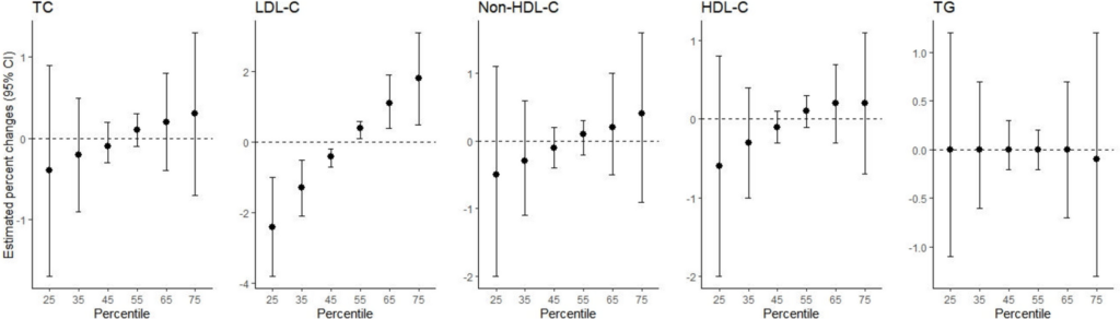
In the BKMR analysis, which flexibly models non-linear exposure–response relationships and interactions among exposures [44], we evaluated the cumulative overall associations between the chemical mixture and lipid levels by predicting outcomes based on simultaneous increases or decreases in all the considered chemicals from their median values. A Gaussian distribution was applied for modeling blood lipid levels in the BKMR models. We also estimated the posterior inclusion probabilities (PIPs) for each pollutant, which indicate the relative importance of individual exposures in contributing to overall effects. A PIP of > 0.5 suggests that the inclusion of an exposure improves the model fit in more than half of the iterations, making it a meaningful predictor. We then explored the associations between individual chemicals and lipid levels, holding the concentrations of all other chemicals constant at the 25th, 50th, and 75th percentiles, respectively. The BKMR models were adjusted for the same set of covariates and implemented using the Markov Chain Monte Carlo method with 10,000 iterations. A hierarchical variable structure was imposed, grouping all PFASs together and all heavy metals together [27]. The BKMR analyses were conducted using the bkmr package in R software.
To complement the supervised machine learning-based BKMR approach, we also applied the k-means clustering method, a widely used unsupervised dimension reduction technique. In the k-means clustering analysis, we identified actual exposure profiles in this population, clustered adolescents with similar pollutant exposure patterns, and linked these clusters (with distinguishable exposure profiles) to health outcomes. We standardized all PFASs and heavy metals into Z-scores, repeated k-means cluster analyses with increasing numbers of clusters, and determined the optimal number of clusters using the cubic cluster criterion (CCC) and pseudo F statistics. Since the CCC and pseudo F statistics decreased continuously when the number of clusters exceeded two (Table S2), we assigned participants into two clusters [45]. We then constructed similar linear regression models, considering the complex survey design and adjusting for the same covariates, while using cluster membership instead of individual chemical levels as exposures. The cluster with the lower chemical exposure profile served as the reference. These analyses were performed using the STANDARD and FASTCLUS procedures in SAS software.
We also conducted analyses for secondary binary outcomes (high TC, high LDL-C, high non-HDL-C, low HDL-C, and high TG) using logistic regression models (the SURVEYLOGISTIC procedure in SAS software) and BKMR models with a probit link function (the bkmr package in R software). For the logistic regression models, we used individual pollutants, as well as the cluster memberships identified from k-means clustering, as exposures. The covariates and model specifications were consistent with those used for continuous lipid level analyses.
We performed gender-stratified analyses and evaluated the interactions between pollutants and gender by testing the product terms of pollutant levels and gender. These analyses were conducted because previous studies have reported gender-specific differences in the health effects of PFAS and heavy metal exposure [39, 40, 45]. Additionally, disruption of sex hormone homeostasis, such as estrogen imbalance, may be one of the underlying mechanisms for the associations of PFASs and heavy metals with lipid levels [40, 45].
We performed several sensitivity analyses to confirm the robustness of the results. First, we repeated the analyses without adjusting for BMI, considering the potential mediating role of BMI. Second, we adjusted for the consumption of big fish and tuna (≤ once/month, 1–3 times/month, or ≥ once/week) instead of total fish intake. Third, we included frozen meal intake (almost none, 1–3 times/month, once/week, or ≥ twice/week) as an additional covariate to account for the overall diet quality, as a comprehensive diet quality index was not available in the KoNEHS dataset. Fourth, we controlled for urine dilution effects using the conventional standardization method (dividing urine chemical levels by urine creatinine levels) instead of the method suggested by O’Brien et al. [46]. This allowed for direct comparison with previous studies that utilized the conventional standardization method. Fifth, we assessed mercury exposure using blood mercury levels, a commonly used biomarker primarily reflecting methylmercury, instead of urine mercury levels. Blood mercury levels were measured using whole blood samples with a gold amalgamation direct mercury analyzer (DMA-80, Milestone, CT, USA), with a LOD of 0.01 μg/L. One participant had a value below the LOD, which was imputed as the LOD divided by the square root of two. Sixth, we created a categorized variable for the covariate-adjusted standardized urine cadmium levels (below the LOD; greater than or equal to the LOD but below the median; and greater than or equal to the median) and evaluated the associations of urine cadmium levels (categorized variable) with blood lipid levels and dyslipidemia using the same linear and logistic regression models, with the ‘below the LOD’ category as the reference.
We presented the results from linear regressions and BKMR analyses with continuous outcomes as percent (%) changes per doubling of concentrations of PFASs and heavy metals, calculated using the formula: (100times ({e}^{upbeta }-1)), where β represents a regression coefficient. For logistic regressions, results were presented as odds ratios (ORs). Since only probit regressions were available for binary outcomes in the BKMR analysis, we presented regression coefficients from probit regressions (βprobit) for the dyslipidemia outcomes. To increase interpretability, we also translated βprobit into the more familiar association estimator of OR using the formula: (ORapprox e^{1.6timesbetatext{probit}}) [47, 48]. All analyses were performed using SAS (version 9.4, SAS Institute Inc.) and R (version 4.3.2, R Development Core Team) software.